


1. Introduction
Response Surface Models, a variation of the simple linear regression, with the incorporation of the second order effects of non-linear relationships, is a popular optimization technique to determine the best possible combinations of variables to determine a specific response to a phenomenon (Minimum/maximum/saddle point).
RSM is particularly useful to understand the relationship between multiple predictor variables with 1 or more predictands.
The technique is popular in industries where process and statistical optimization plays a key role, such as the chemical, enzyme and manufacturing industry, biochemical labs, textile industry etc. Traditional optimization techniques such as the COST (Changing-one-single-thing) or the OFAT (one-factor-at-a-time) techniques are misleading in computing the optimum as they do not take into account factor interactions. Additionally, in real life scenarios, changes in multiple factors impact a specific response. This is where RSM comes in.
In the below scenario, the experiment involves OFAT wise experimentation of the three factors in 15 runs (3 factor* 5 runs each). It can be observed that given the experimental results collected, it is possible to derive linear and quadratic relationship, however, establishing factor interactions is not possible in the given scenario.
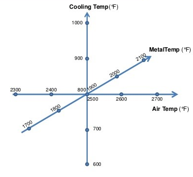
Figure 1: Source: ASQ Reliability Division (Slideshare)
RSM involves sequential experimentation as we look out for an optimum in response. The focus in RSM is to look out for a new factorial that is a good approximation to capture the interactions of a phenomenon.
2. Data
The below pilot was conducted with KPIs associated with the weaving process of a textile mill. The target of the below exercise is to get optimum settings of yarn quality and loom settings to maximize number of meters weaved (/loom yield).
The following are prerequisites for the RSM methodology:
- Independent variables selected must be controllable in nature. Variables that cannot be controlled, though significant, must be kept constant before the experimentation process. This can be done based on a or prior-experience
- Pre-processing such as Outlier treatment, missing value treatment and necessary transformations must be duly performed
- Correlation analysis/step-wise VIF must be subsequently performed to drop the variables that exhibit high correlation with each other (correlation coeff > 0.60 can be dropped)
3. Methodology
Assuming that the prerequisites were met, the following methodology was used to generate an optimum response surface.
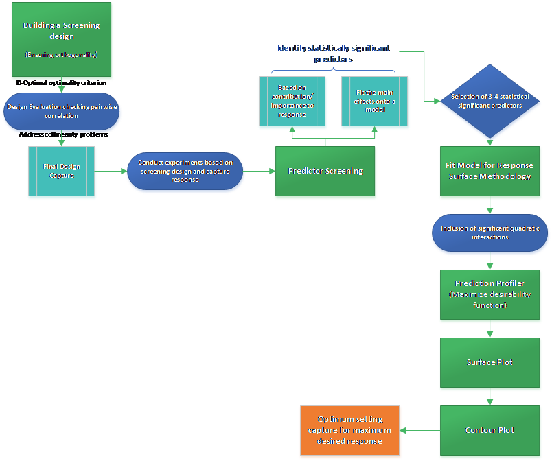
Figure 2: Methodology at a glance
4. Results and Interpretation
4.1 Selection of screening design
The foremost step in the process of Optimum surface determination is the creation of a good screening design based on the data available. In case, historical data is available, a custom design can be created based on the historical data collected. The below screening design is a 2-level full factorial design (with all possible combinations of factors to estimate the main and interaction effects) to define the experimental space.
Number of factors “ n
Number of levels – 2
Number of experimental runs required “ 2<sup>n</sup>
The 2-levels of factors (based on High and Low values) are coded based on realistic range of the factors (Table 1). Corresponding response (meters weaved) must be recorded for each factor combination settings.
Table 1: Table with coded values of 2-level of factors
|
A% |
P |
RPM |
Wp/ph |
WP Eff Loss |
WT tstp |
RunT |
KPICKS |
Lea Strength |
Imperfections |
Hairiness |
Twist Factor |
Elongation |
|
|
Low (-1) |
55 |
70 |
250 |
0 |
4.5 |
2 |
110 |
26 |
7 |
22.67 |
3 |
4 |
3.2 |
|
High (+1) |
70 |
100 |
350 |
9.7 |
5.3 |
4 |
128.5 |
44.2 |
10 |
52.8 |
6 |
8 |
8 |
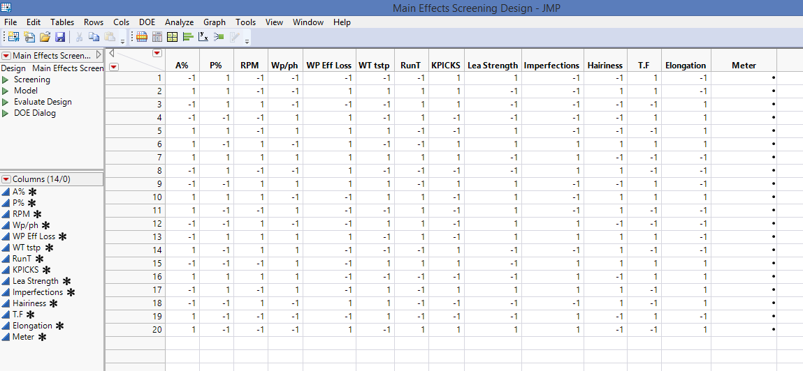
Figure 3: Factorial Design Matrix (Selection of Screening Design)
Note:
- The below design has no replication (running design more than once is easier for data analysis). Replication is essential to ensure the homogeneity of variance across the experimental space by excluding the factor combinations that result in inconsistency in response variables from the factor space.
- Inclusion of center points will improve the final factorial design matrix
The design must be checked for orthogonality by calculating the pair-wise estimate of correlation of factors (Figure 4). Additionally, many algorithms have been developed to calculate the minimum number of runs required to ensure orthogonality to minimize the cost of multiple experimental runs.
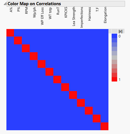
Figure 4: Correlation Plot of screening design
4.2 Predictor Screening
The next step involves identifying the screening of predictors for their ability to predict an outcome. This has been performed using the Predictor Screening in JMP. The screening algorithm uses the bootstrap random forest partitioning technique to evaluate the contribution of predictors on the predictand. Additionally, the predictor screening can identify predictors that might be weak predictors when used alone but strong when used in combination with other predictors. This is especially useful in this methodology, as the interaction element is also taken into account.
An aggressive approach of predictor screening was used in this sample run. In practical situations, however, multiple iterations need to be performed to drop variables. Model performance measures must be checked with each individual iteration.
Below, only the top 4 contributing predictors of the first iteration was selected for the steps ahead. The results of the predictor screening can be verified by fitting a linear model based on the same data. A good predictor will have a p-value < 0.05 (based on the confidence level considered) to be statistically significant.
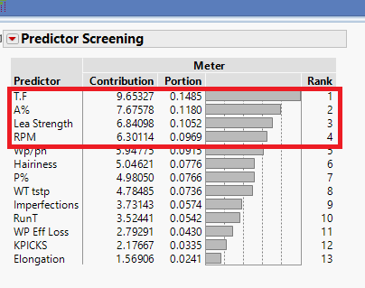
Figure 5: Result of Predictor Screening
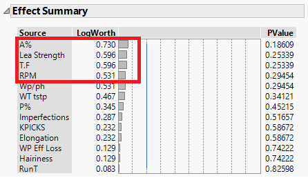
Figure 6: Result of Linear model
4.3 Fitting model for RSM
The next step requires us to fit the selected predictors to an RSM model.
- RSM will estimate the main effect, the interaction effect (cross-linear effect “ XY and quadratic effect “ X<sup>2</sup>)
- The significant effects contributing to the response must be selected based on the results of the ANOVA table
- We may notice aliasing or confounding of the main effects, that can be identified in the alias matrix and the design diagnostics.
X -> Y + XYZ
If multiple-way interactions are noticed to be active and strong, the design can be concluded to be poor and tweaking will be required accordingly.
Prediction profiler is checked to maximize the desirability function by setting maximum meters dyed (loom yield). The procedure helps identify optimum settings for all the contributing variables.
- The controls given in the prediction profiler lets us see how the prediction model changes as the individual settings of predictors are changed
- Model sensitivity can be gauged in the profiler
The maximum yield (21.947 m) with corresponding settings of A%, RPM, Lea Strength & T.F can be observed in Figure 7.
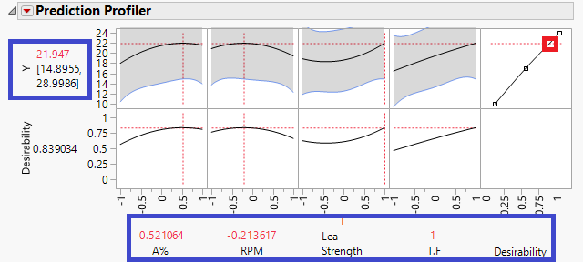
Figure 7: Output of Prediction Profiler
4.4 Visualization of Response Surfaces
Surface Plot and Contour plots help us visualize the response surface in a 2-D and 3-D plot.
The gridded Surface Plot is a representation of the surface plot in a 3-D Space. The plot determining optimum operating conditions reaching maximum from the best-fitted model with a map of contour lines, follows a direction of movement along the path of maximum response from a reference point.
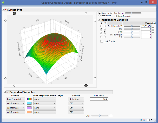
Figure 8: Surface Plot
The gridded Contour Plot generated the contours of a response variable in a rectangular coordinate system as shown in Figure 9. A contour plot shows a 3D surface in two dimensions with contours delineating changes in the 3-D space. The contour lines represent lines of equal response and can be visualized as response contours two factors at a time. The remaining predictors (contributing least to response) are fixed at a given point. In the above example, lea strength and TF have been fixed at 1 based on the results of the prediction profiler.
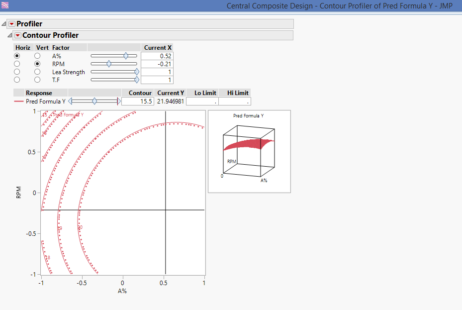
Figure 9: Contour Profiler
Finally, the optimum coded value have to be converted into the uncoded form based on the same high-low transformation. It is recommended to test the model performance based on available validation data or by replicating the results in an actual set-up, if cost is not a restraint.
